데이터를 분류하고 예측하는 결정에 이르기 위해 특정 기준에 따라 'yes/no'로 답할 수 있는 질문을 이어나가면서 학습하는 의사결정나무(DecisionTree)에 대해서 정리해 보자.
이 전의 머신러닝 파트에서는 나이브베이즈 분류를 BernoulliNB를 통해서 실습해 보았다.
[나이브 베이즈 분류Naive Bayes Classification] - BernoulliNB with Python
데이터가 각 클래스에 속할 특징 확률을 계산하는 조건부 확률 기반의 분류 방법인 나이브베이즈(NaiveBayes)에 대해서 정리해 보자. 그중에서 오늘은 BernoulliNB에 대해서 알아볼 것이다. 이 전의 머
py-moon.tistory.com
의사결정나무(DecisionTree)는 원본 데이터에서 하나의 규칙을 만들 때마다 노드를 만들고, 가지를 치면서 내려간다.
그러므로 의사결정나무(DecisionTree)를 통해 얻은 예측 결과는 분류 규칙이 명확하여 해석을 쉽게 할 수 있다.
또한 선형성과 정규성 등의 가정이 필요하지 않아 전처리 과정에 모델의 성능이 큰 영향을 받지 않는다.
따라서, 본 실습에서 별 다른 전처리 과정을 진행하지 않는다.
의사결정나무(DecisionTree)에서 학습의 의미는 '정답에 가장 빨리 도달하는 질문목록을 학습'하는 것이다.
의사결정나무(DecisionTree)는 데이터를 통해 각 마디에서 최적의 분리규칙(Splitting Rule)을 찾아 결정트리의 질문목록을 생성한다.
트리를 성장시키는 과정에서 적절한 정지규칙(Stopping Rule)을 만족하면 자식노드의 생성을 중단한다.
분리규칙을 설정하는 분리기준(Splitting Criterion)은 종속변수가 이산형 데이터인지 연속형 데이터인지에 따라 다르다
종속변수가 이산형 데이터일 때 분류분석을 진행할 수 있다.
이때, 사용하는 기준값에 따른 분리기준은 카이제곱 통계량 p값, 지니지수, 엔트로피 지수가 있다.
그렇다면, UCI Machine Learning 저장소의 독일 신용데이터를 통해 의사결정나무 분류분석을 진행해 보자.
|
1
2
3
4
5
6
7
8
9
10
11
12
13
|
from sklearn.metrics import confusion_matrix, accuracy_score, precision_score, recall_score, f1_score
from sklearn.model_selection import train_test_split
from sklearn.tree import DecisionTreeClassifier
from sklearn.metrics import classification_report
import matplotlib.pyplot as plt
from sklearn.metrics import plot_roc_curve, roc_auc_score
import pandas as pd
import numpy as np
import warnings
warnings.filterwarnings(action='ignore')
credit = pd.read_csv('data/credit_final.csv')
|
cs |
> 분류 분석을 진행하기 위해 필요한 라이브러리와 데이터셋을 불러와준다.
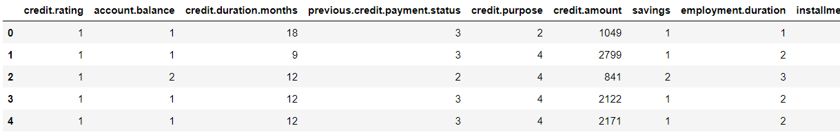
> head()를 이용해서 상위 데이터 5개를 확인할 수 있다.
> 변수명이 길어서 그런지 한 페이지에 다 들어오진 않는다.
|
1
2
3
4
5
6
7
8
9
10
|
from sklearn.model_selection import train_test_split
x = credit.drop(['credit.rating'], axis = 1)
y = credit['credit.rating']
train_x, test_x, train_y, test_y = train_test_split(x, y, stratify = y, test_size = 0.3, random_state = 42)
print(train_x.shape, test_x.shape, train_y.shape, test_y.shape)
(700, 20) (300, 20) (700,) (300,)
|
cs |
> 별도의 전처리를 거치지 않고 모델 학습을 위해 데이터셋을 분리해 준다.
|
1
2
3
4
5
6
|
from sklearn.tree import DecisionTreeClassifier
clf = DecisionTreeClassifier(max_depth = 5)
clf.fit(train_x, train_y)
pred = clf.predict(test_x)
|
cs |
> 본 실습에서 활용할 모델인 DecisionTreeClassifier의 객체를 불러온 다음, 학습을 진행한다.
> pred변수에 예측값을 저장해 놓는다.
|
1
2
3
4
5
6
7
8
9
10
11
12
13
14
15
16
17
18
19
20
21
22
23
|
from sklearn.metrics import confusion_matrix, accuracy_score, precision_score, recall_score, f1_score
test_cm = confusion_matrix(test_y, pred)
test_acc = accuracy_score(test_y, pred)
test_prc = precision_score(test_y, pred)
test_rcll = recall_score(test_y, pred)
test_f1 = f1_score(test_y, pred)
print(test_cm)
print('\n')
print('정확도 : {:.2f}%'.format(test_acc*100))
print('정밀도 : {:.2f}%'.format(test_prc*100))
print('재현율 : {:.2f}%'.format(test_rcll*100))
print('F1-score : {:.2f}%'.format(test_f1*100))
[[ 30 60]
[ 22 188]]
정확도 : 72.67%
정밀도 : 75.81%
재현율 : 89.52%
F1-score : 82.10%
|
cs |
> 모델의 성능을 평가하기 위해 분류 분석에서 사용하는 평가지표를 가져온다.
> 혼동행렬과 더불어 정확도, 정밀도, 재현율을 확인하며 모델의 성능을 파악할 수 있다.
|
1
2
3
4
5
6
7
8
9
10
11
12
13
14
|
from sklearn.metrics import classification_report
report = classification_report(test_y, pred)
print(report)
precision recall f1-score support
0 0.58 0.33 0.42 90
1 0.76 0.90 0.82 210
accuracy 0.73 300
macro avg 0.67 0.61 0.62 300
weighted avg 0.70 0.73 0.70 300
|
cs |
> 추가적으로 classification_report를 통해서 모델에 대한 더 자세한 혼동행렬의 정보를 파악할 수 있다.
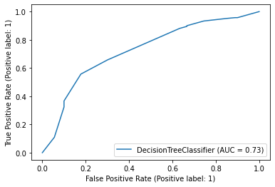
> 분류 분석의 또 다른 평가지표인 ROC곡선과 AUC값을 확인해 볼 수도 있다.
> ROC곡선 그래프에서는 곡선의 정도, AUC값은 1에 가까울수록 성능이 좋다고 해석이 가능하다.
|
1
2
3
4
5
6
7
|
from sklearn.metrics import roc_auc_score
score = roc_auc_score(test_y, clf.predict_proba(test_x)[:, 1])
print('ROC_AUC_score : {:.2f}'.format(score))
ROC_AUC_score : 0.73
|
cs |
> 모델의 predict_proba를 통해서 예측치에 대한 확률을 가져오고, 이를 가지고 roc_auc_score값을 구할 수 있다.
|
1
2
3
4
5
6
7
8
9
10
11
12
13
14
15
16
17
18
19
20
21
22
23
24
25
26
27
28
29
|
importances = clf.feature_importances_
column_nm = pd.DataFrame(x.columns)
feature_importances = pd.concat([column_nm, pd.DataFrame(importances)], axis = 1)
feature_importances.columns = ['feature_nm', 'importances']
print(feature_importances)
feature_nm importances
0 account.balance 0.314978
1 credit.duration.months 0.168067
2 previous.credit.payment.status 0.074265
3 credit.purpose 0.023764
4 credit.amount 0.075771
5 savings 0.111225
6 employment.duration 0.046676
7 installment.rate 0.000000
8 marital.status 0.012202
9 guarantor 0.022279
10 residence.duration 0.000000
11 current.assets 0.012996
12 age 0.103415
13 other.credits 0.018117
14 apartment.type 0.000000
15 bank.credits 0.000000
16 occupation 0.016245
17 dependents 0.000000
18 telephone 0.000000
19 foreign.worker 0.000000
|
cs |
> 트리를 생성하기 전 중요한 변수가 무엇인지 확인하기 위해 변수중요도를 확인한다.
> account.balance변수가 가장 높은 변수중요도를 가진다고 해석할 수 있다.
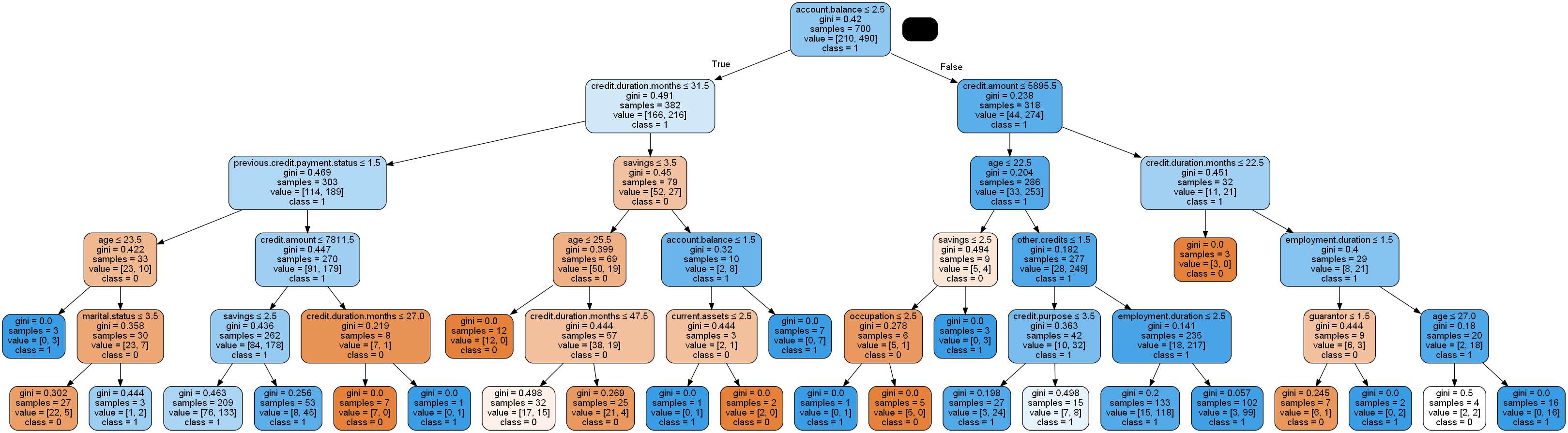
> 위와 같이 의사결정나무의 분류분석의 결과물을 확인할 수 있다.
> 확대해서 보면 지니지수와 샘플 수, 클래스, value값을 확인할 수 있다.
종속변수가 연속형 데이터일 때 회귀분석을 진행할 수 있다.
이때, 사용하는 기준값에 따른 분리기준은 분산분석에서 F통계량, 분산의 감소량이 있다.
그럼, Numpy를 이용해 임의의 데이터를 생성해서 의사결정나무를 이용한 회귀분석을 진행해 보자.
|
1
2
3
4
5
6
7
8
9
10
11
12
13
|
import numpy as np
from sklearn.tree import DecisionTreeRegressor
from sklearn.model_selection import train_test_split
from sklearn.metrics import mean_squared_error, mean_absolute_error
import pandas as pd
import matplotlib.pyplot as plt
np.random.seed(0)
x = np.sort(5 * np.random.rand(400, 1), axis = 0)
T = np.linspace(0, 5, 500)[:, np.newaxis]
y = np.sin(x).ravel()
y[::1] += 1 * (0.5 - np.random.rand(400))
|
cs |
> 회귀 분석을 진행하기에 필요한 라이브러리와 Numpy를 이용해서 임의로 데이터를 생성해 준다.
> 타깃데이터인 y에는 임의로 노이즈를 추가해 준다.
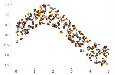
> 임의로 생성한 데이터들의 관계를 알아보기 위해 산점도를 확인해 본다.
|
1
2
3
4
5
6
7
|
from sklearn.model_selection import train_test_split
train_x, test_x, train_y, test_y = train_test_split(x, y, test_size = 0.3, random_state = 42)
print(train_x.shape, test_x.shape, train_y.shape, test_y.shape)
(280, 1) (120, 1) (280,) (120,)
|
cs |
> 의사결정나무 회귀분석의 모델 학습을 위해 데이터를 7:3으로 분할해 준다.
|
1
2
3
4
5
6
7
8
|
reg_1 = DecisionTreeRegressor(max_depth = 2)
y_1 = reg_1.fit(train_x, train_y).predict(test_x)
reg_2 = DecisionTreeRegressor(max_depth = 5)
y_2 = reg_2.fit(train_x, train_y).predict(test_x)
reg_3 = DecisionTreeRegressor(max_depth = 7)
y_3 = reg_3.fit(train_x, train_y).predict(test_x)
|
cs |
> 트리의 최대 깊이를 설정하는 max_depth를 각각 2, 5, 7로 설정하고, 세 모델의 성능을 비교분석해 보자.
|
1
2
3
4
5
6
7
8
9
10
11
12
13
14
15
16
17
18
|
from sklearn.metrics import mean_squared_error, mean_absolute_error
import pandas as pd
import numpy as np
preds = [y_1, y_2, y_3]
weights = ['max_depth = 2', 'max_depth = 5', 'max_depth = 7']
evls = ['MSE', 'RMSE', 'MAE']
results = pd.DataFrame(index = weights, columns = evls)
for pred, nm in zip(preds, weights):
mse = mean_squared_error(test_y, pred)
mae = mean_absolute_error(test_y, pred)
rmse = np.sqrt(mse)
results.loc[nm]['MSE'] = round(mse, 2)
results.loc[nm]['RMSE'] = round(rmse, 2)
results.loc[nm]['MAE'] = round(mae, 2)
|
cs |
> 세 모델에 대해서 오차에 대한 값을 나타내는 성능지표를 통해서 의사결정나무의 성능을 파악해 보자.
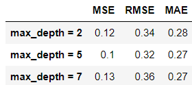
> 결과표를 확인해 보면 max_depth가 5일 때, 예측값과 타깃값과의 오차가 가장 적다고 해석할 수 있다.
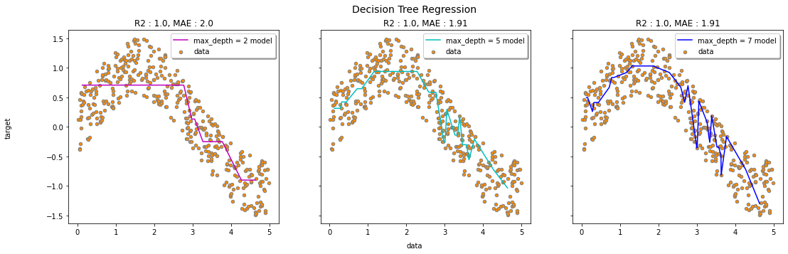
> 세 모델에 대해서 의사결정나무의 예측결과를 시각화해 보았다.
> 세 모델을 비교해 보면 눈에 띄는 차이가 보이진 않지만, 수치로서 겨우 확인할 수 있을 정도다.
OUTTRO.
EDA와 전처리를 진행했다면 십중팔구 현 성능보다 좋은 성능을 가지는 모델을 구축할 수 있다.
하지만, 머신러닝 파트에서 올리는 게시물은 기법을 소개하고 실습을 진행하는 것에 의의를 둔다.
좋은 성능을 가지는 모델을 구축하는 공부를 하지 않는 것은 아니다.
데이콘이나 캐글에서 관련된 온라인 대회가 개최되면 참여하는 편이다.
그리고 다른 카테고리에 보면 지난 분석과제들을 수행하고 기록해 놓은 게시물들이 올라와있다.
머신러닝이나 통계분석에서 습득한 지식을 가지고 분석과제에 써먹곤 한다.
'내가 하는 데이터분석 > 내가 하는 머신러닝' 카테고리의 다른 글
| [나이브 베이즈 분류, Naive Bayes Classification] - BernoulliNB with Python (0) | 2023.02.19 |
|---|---|
| [나이브 베이즈 분류, Naive Bayes Classification] - MultinomialNB with Python (0) | 2023.02.17 |
| [나이브 베이즈 분류, Naive Bayes Classification] - GaussianNB with Python (0) | 2023.02.15 |
| [앙상블, Ensemble] - RandomForest with Python (0) | 2023.02.13 |
| [앙상블, Ensemble] - Boosting with Python (0) | 2023.02.11 |


