이 전엔 DACON-와인 품질 분류 분석과제를 수행해보고 복습해보았다.
DACON - 와인 품질 분류(분류)
두 달 전쯤 처음 데이콘을 접하며 접근하기 쉬운 초급대회를 선정하여 내 수준을 알아보고, 복습도 할 겸 참여해봤다. 그저 아는 만큼만 하려니 어렵지 않았지만 결과는 형편없었다. 그 이후 전
py-moon.tistory.com
|
1
2
3
4
5
6
7
8
9
10
11
12
13
14
15
16
17
18
19
20
21
22
23
24
|
import pandas as pd
import numpy as np
import matplotlib.pyplot as plt
import seaborn as sns
import warnings
warnings.filterwarnings('ignore')
train = pd.read_csv('C:/Users/k1560/Desktop/Bicycle/train.csv')
test = pd.read_csv('C:/Users/k1560/Desktop/Bicycle/test.csv')
submission = pd.read_csv('C:/Users/k1560/Desktop/Bicycle/submission.csv')
# id : 고유id
# hour : 시간
# temperature : 기온
# precipitation : 비가 오지 않았으면 0, 비가 오면 1
# windspeed : 풍속(평균)
# humidity : 습도
# visibility : 시정(視程), 시계(視界)(특정 기상 상태에 따른 가시성을 의미)
# ozone : 오존
# pm10 : 미세먼지(머리카락 굵기의 1/5에서 1/7 크기의 미세먼지)
# pm2.5 : 미세먼지(머리카락 굵기의 1/20에서 1/30 크기의 미세먼지)
# count : 시간에 따른 따릉이 대여 수
print(train.shape, test.shape, submission.shape)
|
cs |
-> 우선, 제공받은 데이터들의 shape을 확인한다.
|
1
2
|
train = train.drop(['id'], axis=1)
test = test.drop(['id'], axis=1)
|
cs |
-> 본격적으로 시작하기에 앞서 필요없는 변수는 우선제거한다.
|
1
2
3
4
5
6
7
8
9
|
train.rename(columns={'hour_bef_temperature':'temperature', 'hour_bef_precipitation':'precipitation',
'hour_bef_windspeed':'windspeed', 'hour_bef_humidity':'humidity',
'hour_bef_visibility':'visibility', 'hour_bef_ozone':'ozone',
'hour_bef_pm10':'pm10', 'hour_bef_pm2.5':'pm2.5'},inplace = True)
test.rename(columns={'hour_bef_temperature':'temperature', 'hour_bef_precipitation':'precipitation',
'hour_bef_windspeed':'windspeed', 'hour_bef_humidity':'humidity',
'hour_bef_visibility':'visibility', 'hour_bef_ozone':'ozone',
'hour_bef_pm10':'pm10', 'hour_bef_pm2.5':'pm2.5'},inplace = True)
|
cs |
-> 변수들의 이름이 불필요하게 길게 되었있어서 추후의 분석에 용이하게 하기위해 미리 변수의 이름을 바꿔준다.
|
1
|
train.isnull().sum()
|
cs |
|
1
2
3
4
5
6
7
8
9
10
|
hour 0
temperature 2
precipitation 2
windspeed 9
humidity 2
visibility 2
ozone 76
pm10 90
pm2.5 117
count 0
|
cs |
-> train데이터셋의 결측치를 확인해보니 꽤 있음에 결측치 대체를 해야만 했다.
|
1
2
3
4
5
6
7
8
9
10
11
|
def med(data, col):
data[col] = data[col].fillna(data[col].median())
return data[col]
cols = ['ozone', 'pm10', 'pm2.5', 'windspeed', 'temperature', 'humidity', 'visibility']
for i in cols:
med(train, i)
med(test, i)
train['precipitation'] = train['precipitation'].fillna(1)
test['precipitation'] = test['precipitation'].fillna(1)
|
cs |
-> 결측값을 가지고 있는 컬럼에 한해서 중위값으로 대체했다.
하지만 precipitation변수는 0과 1로 표현되므로 모두 비가오는 1로 대체하였다.
|
1
2
|
train = train.astype({'precipitation':'int32'})
test = test.astype({'precipitation':'int32'})
|
cs |
-> info를 찍어보니 precipitation변수가 float64형으로 되어있다. 후의 분석을 용이하게 하기위해 int32로 변환해 주었다.
|
1
|
train.corr()
|
cs |
-> train데이터셋의 상관관계를 찍어보았다.
-> 분석 결과 count와 pm10,pm2.5,predipitation은 상관계수가 차례대로 -0.1, -0.12, -0.16로써
상관관계가 없다는 인사이트를 주었지만 직관을 고집하여 삭제하지 않고 그대로 분석을 진행한다.
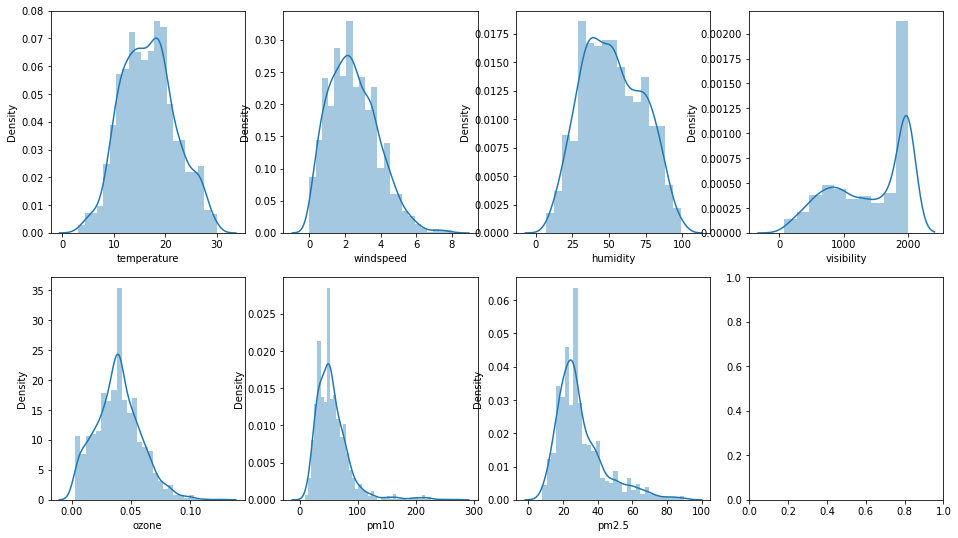
-> 연속형 변수에 대해서 히스토그램을 찍어본 결과 정규화가 필요해보인다.
|
1
|
log_train = np.log1p(train[['temperature','windspeed','humidity','visibility','ozone','pm10','pm2.5']])
|
cs |
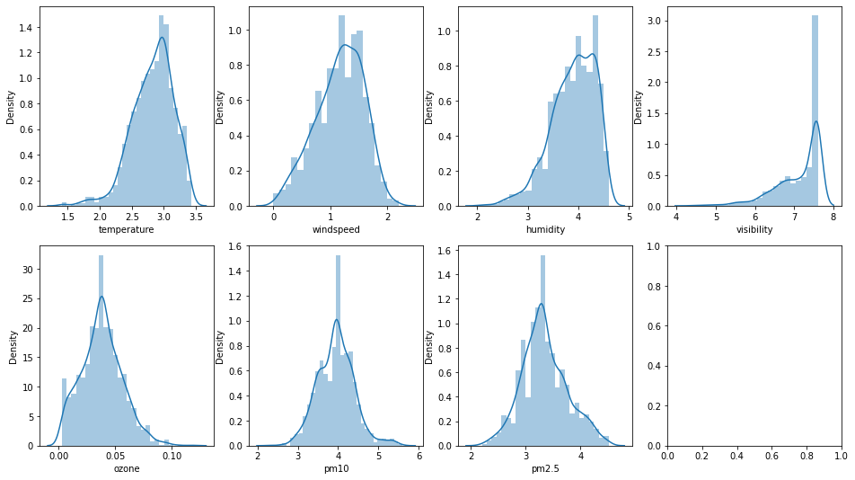
-> 로그변환 후 히스토그램을 다시 찍어보니
pm10과 pm2.5, windspeed는 한 눈에 봐도 정규화가 잘 된걸 확인할 수 있었다.
-> 하지만, 다른 변수에 대해서는 잘 이루어지지 않은게 의문이다. ozone을 제외한 나머지 세 변수는 왜도가 우측으로 쏠린 경향을 보이는 듯 하다.
-> visibility는 시정이 좋은 날이 극도로 많았다고 볼 수 밖엔 없는건가..
|
1
2
|
train_x = train.drop(['count'], axis = 1)
train_y = train['count']
|
cs |
-> 앞서 정제한 데이터들을 가지고 GridSearchCV를 활용하기 전 데이터셋을 나눈다.
|
1
2
3
4
5
6
7
8
9
10
11
12
13
14
|
from sklearn.ensemble import RandomForestRegressor
from sklearn.model_selection import GridSearchCV
params = { 'n_estimators' : [100, 200, 400, 800],
'max_depth' : [14, 16, 18, 20],
'min_samples_leaf' : [1, 3, 5, 7, 9, 11],
'min_samples_split' : [2, 4, 8, 10, 12]}
rfr = RandomForestRegressor(random_state = 2022, n_jobs = -1)
grid_cv = GridSearchCV(rfr, param_grid = params, cv = 3, n_jobs = -1)
grid_cv.fit(train_x, train_y)
print('최적 하이퍼 파라미터:', grid_cv.best_params_)
print('최고 예측 정확도:{:.4f}'.format(grid_cv.best_score_))
|
cs |
-> 모델은 RandomForesetRegressor를 활용할 예정이다.
-> 최적의 하이퍼파라미터를 찾기 위해 GridSearchCV를 사용하였다.
|
1
2
|
최적 하이퍼 파라미터: {'max_depth': 20, 'min_samples_leaf': 1, 'min_samples_split': 2, 'n_estimators': 400}
최고 예측 정확도:0.7668
|
cs |
-> 실행결과로 위와 같이 나왔고 이를 가지고 다시 모델학습을 진행한다.
|
1
2
3
4
5
6
7
8
|
rf_r = RandomForestRegressor(n_estimators = 400,
max_depth = 20,
min_samples_leaf = 1,
min_samples_split = 2,
random_state = 2022,
n_jobs = -1)
rf_r.fit(train_x, train_y)
pred = rf_r.predict(test)
|
cs |
-> 모델학습을 진행하고 test데이터셋을 활용해서 예측된 결과를 pred변수에 할당해줬다.
|
1
2
|
submission['count'] = pred
submission.to_csv('pymoon_bicycle.csv',index = False)
|
cs |
-> 제공된 데이터에 값을 넣어준 채로 저장한 후 파일을 제출한다.
'내가 하는 데이터분석 > 내가 하는 정형 회귀' 카테고리의 다른 글
| [DACON] - 영화 관객수 예측(회귀) with Python (0) | 2023.01.22 |
|---|---|
| [DACON] - FIFA 선수 이적료 예측(회귀) with Python (0) | 2023.01.04 |

