분석 진행 기간 : 2022.12.30 ~ 2023.01.16
INTRO.
최근 통계분석에 정신없이 시간을 보내며 한동안 분석과제에 소홀했다는 생각이 들었다.
이 영화 관객수 예측 과제는 몇 가지 변수의 데이터가 분석에 다루기 까다로운 형태로 되어있어서 데이터 전처리와 EDA에서 가장 많은 시간을 보낸 과제이다.
그래서인지 한 번에 끝내지 않고 긴 시간에 나누어 분석을 진행했다는 핑계로 정리를 하고자 한다.
이전 분석과제에서는 DACON - FIFA 선수 이적료 예측 분석을 진행하며 정리해 보았다.
DACON - FIFA 선수 이적료 예측(회귀) with Python
INTRO. 두 달 전에 FIFA선수 이적료 예측 문제를 풀어본 경험이 있었다. 하지만 이번 기회에 처음으로 돌아가 두 달 전에 놓친 부분이 없었는지를 확인하고 코드를 수정해 보았다. 올린 코드에는 df.
py-moon.tistory.com
DACON - 영화 관객수 예측
|
1
2
3
4
5
6
7
8
9
10
11
12
13
14
15
16
17
18
19
20
21
22
23
24
25
|
import pandas as pd
import numpy as np
import matplotlib.pyplot as plt
import seaborn as sns
import warnings
warnings.filterwarnings('ignore')
train = pd.read_csv('C:/Users/k1560/Desktop/Movie/movies_train.csv')
test = pd.read_csv('C:/Users/k1560/Desktop/Movie/movies_test.csv')
submission = pd.read_csv('C:/Users/k1560/Desktop/Movie/submission.csv')
# title : 영화의 제목
# distributor : 배급사
# genre : 장르
# release_time : 개봉일
# time : 상영시간(분)
# screening_rat : 상영등급
# director : 감독이름
# dir_prev_bfnum : 해당 감독이 이 영화를 만들기 전 제작에 참여한 영화에서의 평균 관객수(단 관객수가 알려지지 않은 영화 제외)
# dir_prev_num : 해당 감독이 이 영화를 만들기 전 제작에 참여한 영화의 개수(단 관객수가 알려지지 않은 영화 제외)
# num_staff : 스텝수
# num_actor : 주연배우수
# box_off_num : 관객수
print(train.shape, test.shape, submission.shape)
|
cs |
> 분석과제에 필요한 라이브러리와 데이터셋을 불러오고, 각 데이터 셋의 길이를 확인한다.
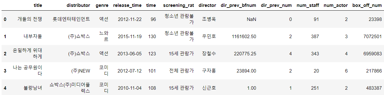
> 데이터의 head()를 찍어보니 결측치도 있고, 날짜 변수도 있고, distributor변수는 전처리가 필요해 보인다는 정도로 확인이 가능하다.
|
1
2
|
train = train.drop(['title', 'director'], axis=1)
test = test.drop(['title', 'director'], axis=1)
|
cs |
> 우선, head()를 찍어본 후 불필요하다고 생각한 변수는 미리 제거한다.
|
1
2
|
train['screening_rat'] = train['screening_rat'].map({'전체 관람가':0, '12세 관람가':1, '15세 관람가':2, '청소년 관람불가':3})
test['screening_rat'] = test['screening_rat'].map({'전체 관람가':0, '12세 관람가':1, '15세 관람가':2, '청소년 관람불가':3})
|
cs |
> screening_rat변수에 순서에 의미가 없는 고윳값이 4개 존재하여 이를 분석에 용이하도록 수치형 변수로 변환한다.
|
1
|
train[['box_off_num']].groupby(train['genre']).mean().sort_values(by = 'box_off_num', ascending = False).T
|
cs |
> 분석을 진행하면서 groupby() 함수를 사용해서 장르별 평균 영화관객 수를 추출해 보았다.

> 결과를 보니 느와르가 편당 평균 약 226만 명, 액션이 편당 평균 약 220만 명, 공상과학이 편당 평균 약 178만 명으로 순위를 보여주고 있다.
|
1
|
train[['box_off_num']].groupby(train['genre']).sum().sort_values(by = 'box_off_num', ascending = False).T
|
cs |
> 이번에는 장르별 총 영화관객 수를 뽑아보았다.

> 결과를 보면 드라마가 약 1억 3827만 명의 관객수로 1위를 차지했고, 코미디가 약 6327만 명의 관객수로 2위, 액션이 약 6171만 명으로 3위를 기록하고 있다.
|
1
|
train[['num_staff']].groupby(train['genre']).mean().sort_values(by = 'num_staff', ascending = False).T
|
cs |
> 마지막으로 장르별 동원된 평균 스태프 수를 조회해 보았다.

> 결과는 후순위로 갈수록 의아한 수치가 기록되고 있지만 역시 인기 장르에서는 수백 명의 스태프가 동원된다는 것을 확인할 수 있었다.
> 물론, 이 수치들은 몇 백개밖에 되지 않는 데이터를 통해 얻은 기초통계량일 뿐이지만 대략적인 순위와 현황은 확인할 수 있다는 점이 데이터분석의 장점이다.
|
1
2
3
4
5
6
7
|
train['release_time'] = pd.to_datetime(train['release_time'])
train['year'] = train['release_time'].dt.year - 2010
train = train.drop(['release_time'], axis=1)
test['release_time'] = pd.to_datetime(test['release_time'])
test['year'] = test['release_time'].dt.year - 2010
test = test.drop(['release_time'], axis=1)
|
cs |
> 다시 돌아와서, 연-월-일로 표시되어 있는 release_time변수에서 연도만 year변수로 추출한 후 release_time변수는 제거한다.
> 그리고 추출한 연도에서 2010을 빼서 데이터 간에 차이는 유지하되, 그 수치가 쓸데없이 커서 유발하는 오류를 방지한다.
|
1
2
3
4
|
train['genre'] = train['genre'].map({'드라마':1, '코미디':2, '액션':3, '느와르':4, '멜로/로맨스':5, '공포':6, 'SF':7,
'미스터리':8, '다큐멘터리':9, '애니메이션':10, '서스펜스':11, '뮤지컬':12})
test['genre'] = test['genre'].map({'드라마':1, '코미디':2, '액션':3, '느와르':4, '멜로/로맨스':5, '공포':6, 'SF':7,
'미스터리':8, '다큐멘터리':9, '애니메이션':10, '서스펜스':11, '뮤지컬':12})
|
cs |
> 위에서 추출해 본 장르별 총 영화관객 수 결과를 참고하여 관객수가 높은 순서대로 수치형 변수로 변환해 주었다.
|
1
2
3
4
5
6
|
import re
train['distributor'] = train.distributor.str.replace("(주)", '')
train['distributor'] = [re.sub(r'[^0-9a-zA-Z가-힣]', '', x) for x in train.distributor]
test['distributor'] = test.distributor.str.replace("(주)", '')
test['distributor'] = [re.sub(r'[^0-9a-zA-Z가-힣]', '', x) for x in test.distributor]
|
cs |
> distributor변수에서 "(주)"라는 키워드를 제거하는 방법이다.
> 그리고 정규 표현식을 이용한 문자열 치환하는 방법을 사용해서 불필요한 키워드를 제거한다.
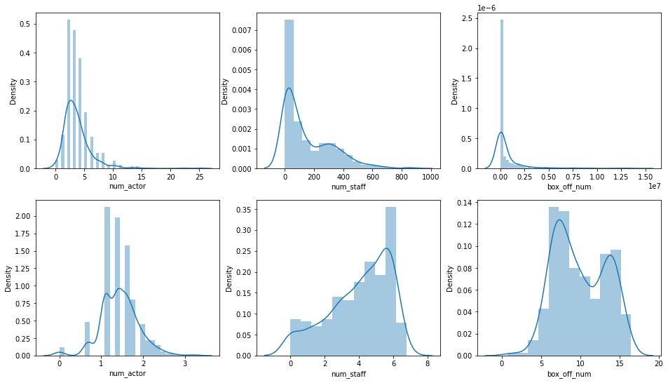
> 다음은 데이터 정규화를 위해 세 변수를 추려내서 각각 np.log1p()를 진행해 주었다.
> 위에 셋은 변환 전, 아래 셋은 변환 후이다.
|
1
2
3
4
5
|
train['num_staff'] = np.log1p(train['num_staff'])
train['num_actor'] = np.log1p(train['num_actor'])
test['num_staff'] = np.log1p(test['num_staff'])
test['num_actor'] = np.log1p(test['num_actor'])
|
cs |
> 결과를 비교하면서 효과를 보는 듯한 두 변수만 로그변환을 해주기로 했다.
|
1
2
|
train['dir_prev_bfnum'] = train['dir_prev_bfnum'].fillna(0)
test['dir_prev_bfnum'] = test['dir_prev_bfnum'].fillna(0)
|
cs |
> 해당 감독이 이 영화를 만들기 전 제작에 참여한 영화에서의 평균 관객수 변수에서 결측값이 파악이 되었고, 0으로 결측값을 제거했다.
|
1
2
3
4
5
|
train = train.drop(['distributor'], axis=1)
test = test.drop(['distributor'], axis=1)
train = train.drop(['year'], axis=1)
test = test.drop(['year'], axis=1)
|
cs |
> 다루기 까다로웠던 distributor 변수와 상관계수가 너무 낮은 year 변수를 제거했다.
> 이로써 길었던 전처리와 EDA를 마무리하고, 모델링을 진행해 보자.
모델링
독립변수 : genre, time, screening_rat, dir_prev_bfnum, dir_prev_bfnum, num_staff, num_actor
종속변수 : box_off_num
|
1
2
3
4
5
6
7
8
9
10
11
12
13
14
15
16
17
18
19
|
from sklearn.model_selection import cross_val_score
from lightgbm import LGBMRegressor
train_x = train.drop(['box_off_num'], axis=1)
train_y = train['box_off_num']
lgbm = LGBMRegressor(random_state = 2022)
# cross_val_score( )로 5 Fold 셋으로 MSE 를 구한 뒤 이를 기반으로 다시 RMSE 구함.
neg_mse_scores = cross_val_score(lgbm, train_x, train_y, scoring="neg_mean_squared_error", cv = 10)
rmse_scores = np.sqrt(-1 * neg_mse_scores)
avg_rmse = np.mean(rmse_scores)
print('LGBMRegressor 10-folds의 개별 RMSE : ', np.round(rmse_scores, 2))
print('LGBMRegressor 10-folds의 평균 RMSE : {0:.3f} '.format(avg_rmse))
LGBMRegressor 10-folds의 개별 RMSE : [ 888780.94 1330410.59 1572298.57 1083113.66 999108.75 1196410.11
2123931.09 1931045.78 2188616.28 1376854.16]
LGBMRegressor 10-folds의 평균 RMSE : 1469056.993
|
cs |
> 위에서 사용한 모델은 LGBMRegressor이다.
> 모델 학습을 위해 데이터셋을 분할해 주고, 모델 객체를 불러와준다.
> 검증할 지표로 RMSE를 사용할 예정이라 scoring을 조정해 준다.
> 출력되는 값은 10번의 교차검증을 한 후 도출된 RMSE와 평균 RMSE를 도출해 낸다.
> 위와 같은 과정을 총 4개의 모델에 동일하게 적용하고 결과를 비교하여 성능이 우수한 모델로 선정하고자 한다.
|
1
2
3
4
5
6
7
8
9
10
11
12
13
14
15
16
17
18
|
from sklearn.model_selection import cross_val_score
from catboost import CatBoostRegressor
train_x = train.drop(['box_off_num'], axis=1)
train_y = train['box_off_num']
cbr = CatBoostRegressor(random_state = 2022)
neg_mse_scores = cross_val_score(cbr, train_x, train_y, scoring="neg_mean_squared_error", cv = 10)
rmse_scores = np.sqrt(-1 * neg_mse_scores)
avg_rmse = np.mean(rmse_scores)
print('CatBoostRegressor 10-folds의 개별 RMSE : ', np.round(rmse_scores, 2))
print('CatBoostRegressor 10-folds의 평균 RMSE : {0:.3f} '.format(avg_rmse))
CatBoostRegressor 10-folds의 개별 RMSE : [1073503.31 1340093.02 1692456.58 1321680.1 1058956.67 1257415.8
2135045.04 1884676.33 2301839.05 1654693.68]
CatBoostRegressor 10-folds의 평균 RMSE : 1572035.959
|
cs |
> 두 번째로 CatBoostRegressor 모델이다.
|
1
2
3
4
5
6
7
8
9
10
11
12
13
14
15
16
17
18
|
from sklearn.model_selection import cross_val_score
from ngboost import NGBRegressor
train_x = train.drop(['box_off_num'], axis=1)
train_y = train['box_off_num']
ngb = NGBRegressor(random_state = 2022)
neg_mse_scores = cross_val_score(ngb, train_x, train_y, scoring="neg_mean_squared_error", cv = 10)
rmse_scores = np.sqrt(-1 * neg_mse_scores)
avg_rmse = np.mean(rmse_scores)
print('NGBRegressor 10-folds의 개별 RMSE : ', np.round(rmse_scores, 2))
print('NGBRegressor 10-folds의 평균 RMSE : {0:.3f} '.format(avg_rmse))
NGBRegressor 10-folds의 개별 RMSE : [1016571.08 1365176.97 1730030.6 1327987.6 1014703.87 1281392.77
1955261.59 1974397.94 2414831.84 1444334.85]
NGBRegressor 10-folds의 평균 RMSE : 1552468.911
|
cs |
> 세 번째는 NGBRegressor 모델이다.
|
1
2
3
4
5
6
7
8
9
10
11
12
13
14
15
16
17
18
|
from sklearn.model_selection import cross_val_score
from sklearn.ensemble import RandomForestRegressor
train_x = train.drop(['box_off_num'], axis=1)
train_y = train['box_off_num']
rfr = RandomForestRegressor(random_state = 2022)
neg_mse_scores = cross_val_score(rfr, train_x, train_y, scoring="neg_mean_squared_error", cv = 10)
rmse_scores = np.sqrt(-1 * neg_mse_scores)
avg_rmse = np.mean(rmse_scores)
print('RandomForestRegressor 10-folds의 개별 RMSE : ', np.round(rmse_scores, 2))
print('RandomForestRegressor 10-folds의 평균 RMSE : {0:.3f} '.format(avg_rmse))
RandomForestRegressor 10-folds의 개별 RMSE : [ 991005.01 1215473.22 1590607.15 1243143.37 989416.22 1317580.82
2005688.2 2131129.54 2238926.34 1460366. ]
RandomForestRegressor 10-folds의 평균 RMSE : 1518333.587
|
cs |
> 마지막으로 RandomForestRegressor모델이다.
|
1
2
3
4
5
6
7
8
9
10
11
12
13
14
15
16
17
18
19
20
21
22
23
|
from lightgbm import LGBMRegressor
from sklearn.model_selection import GridSearchCV
from sklearn.model_selection import KFold
kfold = KFold(n_splits=3, shuffle = True)
params = { 'max_depth' : [3, 5, 7, 9, 11, 13],
'num_iterations' : [100, 200, 400, 800, 1000],
'learning_rate' : [0.01, 0.02, 0.04, 0.08, 0.1],
'num_leaves' : [32, 50, 64, 80, 96, 108],
'boosting' : ['dart']}
lgbm = LGBMRegressor(random_state = 2022, n_jobs = -1)
grid_cv = GridSearchCV(lgbm, param_grid = params, cv = kfold, n_jobs = -1, scoring = 'neg_root_mean_squared_error')
grid_cv.fit(train_x, train_y)
print('최적 하이퍼 파라미터:', grid_cv.best_params_)
print('최고 예측 정확도:{:.4f}'.format(grid_cv.best_score_))
[LightGBM] [Warning] boosting is set=dart, boosting_type=gbdt will be ignored. Current value: boosting=dart
최적 하이퍼 파라미터: {'boosting': 'dart', 'learning_rate': 0.01, 'max_depth': 9, 'num_iterations': 1000, 'num_leaves': 32}
최고 예측 정확도:-1442047.3778
|
cs |
> 성능을 비교해 보니 LGBMRegressor가 가장 적절하다 판단하여 GridSearchCV와 KFold를 사용해서 성능을 더 높일 수 있는 최적의 하이퍼 파라미터를 찾는 과정을 진행했다.
> 결과를 통해서 하이퍼파라미터를 조정한 후에 아래 코드와 같이 예측치까지 추출하였다.
|
1
2
3
4
5
6
7
8
|
from lightgbm import LGBMRegressor
lgbm = LGBMRegressor(random_state = 2022, n_jobs = -1, boosting = 'dart',
learning_rate = 0.01, max_depth = 9, num_iterations = 1000, num_leaves = 32)
lgbm.fit(train_x, train_y)
lgbm_pred = lgbm.predict(test)
#====================================================
submission['box_off_num'] = lgbm_pred
submission.to_csv('pymoon_movie.csv', index=False)
|
cs |
> 제출
OUTTRO.
이번 분석이 공모전 이후로 제일 까다로운 분석이었다.
전처리가 너무 힘들어서 EDA에는 신경을 거의 못 썼다.
제일 까다로웠던 게 distributor 변수를 전처리하는 과정이었는데 이 변수를 써야 할지 말아야 할지부터 고민이었다.
중간중간 groupby() 함수를 쓰면서 카테고리별 인사이트를 도출해 보는 것을 도전해 봤는데 해볼 만한 것 같다.
DACON에 베이스라인 코드를 가끔 참고하는 편인데, 처음 보는 알고리즘으로 결과를 도출해서 꽤 훌륭한 성능을 내는 경우를 봤다. 코드를 이해하진 못했어서 사용하진 않았는데 꽤나 복잡한 프로세스를 갖추고 있었다.
이해할 수만 있다면 내 것으로 만들어 사용할 수 있겠지만.. 좀 더 들여다볼 필요성을 느낀다.
'내가 하는 데이터분석 > 내가 하는 정형 회귀' 카테고리의 다른 글
| [DACON] - FIFA 선수 이적료 예측(회귀) with Python (0) | 2023.01.04 |
|---|---|
| [DACON] - 서울시 따릉이 대여량 예측(회귀) with Python (0) | 2022.12.16 |

