INTRO.
두 달 전에 FIFA선수 이적료 예측 문제를 풀어본 경험이 있었다.
하지만 이번 기회에 처음으로 돌아가 두 달 전에 놓친 부분이 없었는지를 확인하고 코드를 수정해 보았다.
올린 코드에는 df.head(), df.info(), df.describe(), df.shape, df.isnull(), 등등 데이터 이해를 위한 기초 통계량이나 정보에 대해서 확인하는 코드가 생략이 되어있다.
난 이러한 부분에 대해선 전처리나 EDA를 진행하면서도 수시로 찍어보면서 확인해야 하는 부분이라고 생각한다.
상기 이유로 넣지 않았다.
이 전글에선 DACON-타이타닉 생존 예측 분석과제를 수행하고 정리해 보며 다뤄보았다.
DACON - 타이타닉 생존 예측(분류)
분석 진행 기간 : 2022.12.21 ~ 2022.12.31 INTRO. 타이타닉 생존자 예측하는 분석과제는 올해 초에 캐글을 처음 접하면서 처음 해본 분석과제로 기억한다. 지금 하는 분석과의 차이점이 있다면 그땐 주
py-moon.tistory.com
|
1
2
3
4
5
6
7
8
9
10
11
12
13
14
15
16
17
18
19
20
|
import pandas as pd
import numpy as np
train = pd.read_csv('C:/Users/k1560/Desktop/FIFA/FIFA_train.csv')
test = pd.read_csv('C:/Users/k1560/Desktop/FIFA/FIFA_test.csv')
submission = pd.read_csv('C:/Users/k1560/Desktop/FIFA/submission.csv')
# age : 나이
# continent : 선수들의 국적이 포함되어 있는 대륙입니다
# contract_until : 선수의 계약기간이 언제까지인지 나타내어 줍니다
# position : 선수가 선호하는 포지션입니다. ex) 공격수, 수비수 등
# prefer_foot : 선수가 선호하는 발입니다. ex) 오른발
# reputation : 선수가 유명한 정도입니다. ex) 높은 수치일 수록 유명한 선수
# stat_overall : 선수의 현재 능력치 입니다.
# stat_potential : 선수가 경험 및 노력을 통해 발전할 수 있는 정도입니다.
# stat_skill_moves : 선수의 개인기 능력치 입니다.
# value : FIFA가 선정한 선수의 이적 시장 가격 (단위 : 유로) 입니다
print(train.shape, test.shape, submission.shape)
|
cs |
> 필요한 코드, 데이터 불러오기
> 그런 다음 선수의 계약기간을 나타내는 컬럼을 찍어보니 형태(연, 월 연, 일 월 연)가 제각각이었다.
> 따라서, 이를 분석에 용이한 상태로 변환해주기로 한다.
|
1
2
3
4
5
6
|
def year(x):
string = x[-4:]
return int(string)
train['contract_until'] = train['contract_until'].apply(year)
test['contract_until'] = test['contract_until'].apply(year)
|
cs |
> 위 함수는 형태가 제각각인 데이터에서 연도만을 추출할 수 있는 코드로서 데이콘의 베이스라인 코드를 참고하였다.
> train, test데이터셋에 각각 함수를 적용시켜 데이터를 변환해 준다.
|
1
2
3
4
5
|
train['stat'] = (train['stat_overall'] + train['stat_potential'])/2
train = train.drop(['stat_overall', 'stat_potential'], axis=1)
test['stat'] = (test['stat_overall'] + test['stat_potential'])/2
test = test.drop(['stat_overall', 'stat_potential'], axis=1)
|
cs |
> 컬럼 중 선수의 현재 능력치와 선수가 경험 및 노력을 통해 발전할 수 있는 정도를 나타내는 변수가 있는데 둘 다 수치형 데이터이고, 성격이 비슷하다고 판단하여 두 컬럼의 평균으로 stat이라는 변수를 두어 하나의 변수로 함축시켜 준다.
|
1
2
3
4
5
6
7
8
9
10
11
|
position_train = pd.get_dummies(train['position'])
position_test = pd.get_dummies(test['position'])
prefer_foot_train = pd.get_dummies(train['prefer_foot'])
prefer_foot_test = pd.get_dummies(test['prefer_foot'])
train = train.drop(['position', 'prefer_foot'], axis = 1)
test = test.drop(['position', 'prefer_foot'], axis = 1)
train = pd.concat([train, position_train, prefer_foot_train], axis = 1)
test = pd.concat([test, position_test, position_test], axis = 1)
|
cs |
> 범주형 변수를 수치형 변수로 인코딩을 해야 했고, 그 방법으로는 pd.get_dummies를 사용했다.
> 이유는 position, prefer_foot변수 모두 고윳값이 몇 개 없었고, 순서에 의미가 없는 변수였기 때문이다.
|
1
2
3
4
5
|
train = train.drop(['left', 'right'], axis = 1)
test = test.drop(['left', 'right'], axis = 1)
train['contract_until'] = train['contract_until'] - 2018
test['contract_until'] = test['contract_until'] - 2018
|
cs |
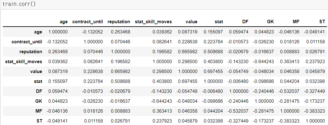
> 모델링을 진행하기 전 확인해본 변수들의 상관계수이다.
> 선수들의 포지션이 생각보다 낮은 상관관계를 가지고 있어서 제거할까도 고민했지만 그렇게 되면 남아있는 독립변수가 몇 없어서 성능에서 문제가 될 수도 있다고 판단했다.
이제 모델링을 진행해보고자 한다.
|
1
2
3
4
5
6
7
8
9
10
11
12
13
14
15
16
17
|
from sklearn.model_selection import cross_val_score
from lightgbm import LGBMRegressor
train_x = train.drop(['value'], axis=1)
train_y = train['value']
lgbm = LGBMRegressor(random_state = 2022, max_depth = 4, n_estimators = 1000)
neg_mse_scores = cross_val_score(lgbm, train_x, train_y, scoring="neg_mean_squared_error", cv = 10)
rmse_scores = np.sqrt(-1 * neg_mse_scores)
avg_rmse = np.mean(rmse_scores)
print('LGBMRegressor 10-folds의 개별 RMSE : ', np.round(rmse_scores, 2))
print('LGBMRegressor 10-folds의 평균 RMSE : {0:.3f} '.format(avg_rmse))
LGBMRegressor 10-folds의 개별 RMSE : [13008635.5 1910972.78 1189299.56 1018455.71 739424.05 598661.92
403917.14 298823.18 227193.95 138299.69]
LGBMRegressor 10-folds의 평균 RMSE : 1953368.347
|
cs |
> 이번 분석 과제에서는 모델을 학습하는 과정과 동시에 교차검증을 진행하는 cross_val_score를 이용해 보았다. line-by-line으로 설명하자면
> 4,5,6줄은 데이터셋을 나누고, 모델을 불러와 객체에 할당시킨 코드이다.
> 8줄에선 cross_val_score에 객체, 데이터, 그리고 검증할 지표로 neg_mean_squared_error를 선택했고, 총 10번의 교차검증을 실시하겠다는 코드이다.
> 9,10줄에서는 음수값으로 나온 neg_mean_squared_error를 양수로 바꾸꿔주면서 RMSE로 변환해 주는 코드와 10번의 교차검증을 통해 나온 10개의 RMSE의 평균을 산출하는 코드이다.
> 모델링에서 총 6가지의 모델을 가지고 위와 동일한 과정을 거쳐 성능을 평가하여, 가장 이상적인 모델을 선정할 예정이다.
> 위에서 다루었던 모델은 LGBMRegressor이며 평균 RMSE는 약 1,953,368이다.
|
1
2
3
4
5
6
7
8
9
10
11
12
13
14
15
16
17
|
from sklearn.model_selection import cross_val_score
from catboost import CatBoostRegressor
train_x = train.drop(['value'], axis=1)
train_y = train['value']
cbr = CatBoostRegressor(random_state = 2022, silent = True, depth = 3)
neg_mse_scores = cross_val_score(cbr, train_x, train_y, scoring="neg_mean_squared_error", cv = 10)
rmse_scores = np.sqrt(-1 * neg_mse_scores)
avg_rmse = np.mean(rmse_scores)
print('CatBoostRegressor 10-folds의 개별 RMSE : ', np.round(rmse_scores, 2))
print('CatBoostRegressor 10-folds의 평균 RMSE : {0:.3f} '.format(avg_rmse))
CatBoostRegressor 10-folds의 개별 RMSE : [12582577.9 1807390.15 1151112.44 1011968.12 748917.03 596311.94
397869.87 299892.31 227215.45 168293.81]
CatBoostRegressor 10-folds의 평균 RMSE : 1899154.901
|
cs |
> 위에서 다루었던 모델은 CatBoostRegressor이며 평균 RMSE는 약 1,899,154이다.
|
1
2
3
4
5
6
7
8
9
10
11
12
13
14
15
16
17
|
from sklearn.model_selection import cross_val_score
from sklearn.ensemble import GradientBoostingRegressor
train_x = train.drop(['value'], axis=1)
train_y = train['value']
gbr = GradientBoostingRegressor(random_state = 2022, max_depth = 5)
neg_mse_scores = cross_val_score(gbr, train_x, train_y, scoring="neg_mean_squared_error", cv = 10)
rmse_scores = np.sqrt(-1 * neg_mse_scores)
avg_rmse = np.mean(rmse_scores)
print('GradientBoostingRegressor 10-folds의 개별 RMSE : ', np.round(rmse_scores, 2))
print('GradientBoostingRegressor 10-folds의 평균 RMSE : {0:.3f} '.format(avg_rmse))
GradientBoostingRegressor 10-folds의 개별 RMSE : [12310325.59 1930504.09 1193334.75 1014990.94 736058.96 598893.89
396353.65 298661.06 223971.44 140414.25]
GradientBoostingRegressor 10-folds의 평균 RMSE : 1884350.863
|
cs |
> 위에서 다루었던 모델은 GradientBoostingRegressor이며 평균 RMSE는 약 1,884,350이다.
|
1
2
3
4
5
6
7
8
9
10
11
12
13
14
15
16
17
|
from sklearn.model_selection import cross_val_score
from ngboost import NGBRegressor
train_x = train.drop(['value'], axis=1)
train_y = train['value']
ngb = NGBRegressor(random_state = 2022, verbose = 500, n_estimators = 500)
neg_mse_scores = cross_val_score(ngb, train_x, train_y, scoring="neg_mean_squared_error", cv = 10)
rmse_scores = np.sqrt(-1 * neg_mse_scores)
avg_rmse = np.mean(rmse_scores)
print('NGBRegressor 10-folds의 개별 RMSE : ', np.round(rmse_scores, 2))
print('NGBRegressor 10-folds의 평균 RMSE : {0:.3f} '.format(avg_rmse))
NGBRegressor 10-folds의 개별 RMSE : [12468261.06 1935536.03 1194364.14 1005048.65 736179.24 583756.16
390974.17 289621.2 227343.71 222751.25]
NGBRegressor 10-folds의 평균 RMSE : 1905383.562
|
cs |
> 위에서 다루었던 모델은 NGBRegressor모델이며 평균 RMSE는 약 1,905,383이다.
|
1
2
3
4
5
6
7
8
9
10
11
12
13
14
15
16
17
|
from sklearn.model_selection import cross_val_score
from sklearn.ensemble import RandomForestRegressor
train_x = train.drop(['value'], axis=1)
train_y = train['value']
rfr = RandomForestRegressor(random_state = 2022, n_estimators = 150)
neg_mse_scores = cross_val_score(rfr, train_x, train_y, scoring="neg_mean_squared_error", cv = 10)
rmse_scores = np.sqrt(-1 * neg_mse_scores)
avg_rmse = np.mean(rmse_scores)
print('RandomForestRegressor 10-folds의 개별 RMSE : ', np.round(rmse_scores, 2))
print('RandomForestRegressor 10-folds의 평균 RMSE : {0:.3f} '.format(avg_rmse))
RandomForestRegressor 10-folds의 개별 RMSE : [12789366.82 2130961.29 1314474.08 1030120.4 739988.87 638695.24
431781.16 318884.32 233863.79 125778.09]
RandomForestRegressor 10-folds의 평균 RMSE : 1975391.406
|
cs |
> 위에서 다루었던 모델은 RandomForestRegressor모델이며 평균 RMSE는 약 1,975,391이다.
|
1
2
3
4
5
6
7
8
9
10
11
12
13
14
15
16
17
|
from sklearn.model_selection import cross_val_score
from xgboost import XGBRegressor
train_x = train.drop(['value'], axis=1)
train_y = train['value']
xgb = XGBRegressor(random_state = 2022, max_depth = 3)
neg_mse_scores = cross_val_score(xgb, train_x, train_y, scoring="neg_mean_squared_error", cv = 10)
rmse_scores = np.sqrt(-1 * neg_mse_scores)
avg_rmse = np.mean(rmse_scores)
print('XGBRegressor 10-folds의 개별 RMSE : ', np.round(rmse_scores, 2))
print('XGBRegressor 10-folds의 평균 RMSE : {0:.3f} '.format(avg_rmse))
XGBRegressor 10-folds의 개별 RMSE : [12126517.2 1896610.74 1209249.47 1004708.11 748441.59 588134.44
396021.83 307297.37 230011.12 193237.43]
XGBRegressor 10-folds의 평균 RMSE : 1870022.930
|
cs |
> 위에서 다루었던 모델은 XGBRegressor모델이며 평균 RMSE는 약 1,870,022이다.
글을 정리하면서 생각난 아이디어로 그때그때 다시 돌려보았을 때 지금보다는 RMSE가 150만 대로 낮아지긴 했지만 개인적으로 만족하지 못하는 결과이다.
총 6가지의 모델을 가지고 성능을 평가해 보았다. 가장 최근에 돌려본 결과로는 CatBoostRegressor모델이 가장 RMSE가 좋게 나왔으며 최종모델로 선정하기로 했다.
|
1
2
3
4
|
from catboost import CatBoostRegressor
cbr = CatBoostRegressor(random_state = 2022, silent = True, depth = 3)
cbr.fit(train_x, train_y)
cbr_pred = cbr.predict(test)
|
cs |
> CatBoostRegressor모델을 다시 학습시키고 예측치까지 cbr_pred에 가져온다.
|
1
2
|
submission['value'] = cbr_pred
submission.to_csv('pymoon_fifa.csv', index=False)
|
cs |
> 제공된 파일에 cbr_pred를 넣고 제출한다.
> 그래도 제출된 파일의 RMSE는 865,411로 나와서 과소적합을 의심해 본다.
OUTTRO.
이번 분석을 하면서 모델링을 진행할 때 모델을 선정하는 과정에서 각각의 모델들이 가지는 특성과 강점, 약점이 있는데 내가 그런 이론적인 부분은 간과하며 모델을 쓰려했다는 점이 부끄럽게 느껴졌다.
ADsP, 빅데이터 분석기사, ADP 필기시험가지 패스 한 지금 상황에서 기본적인 부분을 생각지도 않는 채 그저 문제를 푸는 데에만 집중했던 것 같다.
기본에 충실하지 않은 채 좋은 결과를 내려하는 어리석은 생각과 행동을 한 부분에 대해서 반성하며 다음 분석과제에 임할 것이다.
'내가 하는 데이터분석 > 내가 하는 정형 회귀' 카테고리의 다른 글
| [DACON] - 영화 관객수 예측(회귀) with Python (0) | 2023.01.22 |
|---|---|
| [DACON] - 서울시 따릉이 대여량 예측(회귀) with Python (0) | 2022.12.16 |

